Snowpipe is a continuous data ingestion utility provided by the Snowflake Data Cloud that allows users to initiate any size load, charging their account based on actual compute resource usage.
With this pricing model, you only pay for what you use but the trouble is, it can make it difficult for users to estimate Snowpipe credit consumption for their continuous data ingestion workloads.
In this blog, we will walk you through the Snowpipe credit computation so you and your team can easily calculate and estimate your continuous data ingestion and total cost of ownership (TCO). Additionally, we’ll throw in a few best practices to help you optimize your credit consumption.
PRO TIP: If you’re looking for best practices around How to Optimize Snowpipe Data Load, we highly recommend you check out our other Snowpipe blog!
How are Snowpipe Charges Calculated?
In the Snowpipe serverless compute model, Snowflake provides and manages the compute resources. The compute automatically scales based on the workload. Your continuous ingestion workload may have a very wide table with no transformation or a narrow table with reordering columns and transformation while executing a copy command. Snowflake tracks the resource consumption of loads for your pipe object with per-second/per-core granularity as data load notification actively queues and processes data files. Per-core refers to the physical CPU cores in a compute server. The utilization recorded is then translated into familiar Snowflake credits.
Besides serverless resource consumption, an overhead is included in the utilization costs charged for Snowpipe: 0.06 credits per 1,000 files. This overhead is charged regardless of the event notifications or REST API calls resulting in data being loaded.
Continuous Data Ingestion Workload & Key Metrics
To understand the snowpipe credit consumption, we will go through different workloads as per the following table:
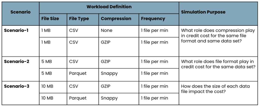
We have taken the most commonly used file formats like CSV (uncompressed or compressed) and Parquet for Snowpipe credit consumption.
We will consider a structured-data set having approximately 40 columns for our simulation. The scenario-1 will place 1Mb of the single CSV data file into stage location by applying compression None and GZIP respectively.
Scenario-2 will load 5Mb of delta data and we will use GZIP compression for CSV and snappy for Parquet and review the performance and credit consumption.
The last scenario, scenario-3, will load 10Mb of delta data with CSV/GZIP and Parquet/snappy file format and compression and review the performance and credit consumption.
To understand and validate the average credit cost, load latency, and overall load performance per scenario per workload, the continuous data loading will run for a 30-60min duration.
Snowpipe Auto Ingest Flow for Continuous Data Load
The data integration pipeline will continuously load data to the cloud storage location where you have set up your Snowflake integration object. The notification services (Event Grid) will notify the pipe object and it will execute a copy command to load the data.

Code Set
					create storage integration azure_int
  type = external_stage
 storage_provider = azure
  	enabled = true
  	azure_tenant_id = '<tenant_id>'
  	storage_allowed_locations = ('azure://myaccount.blob.core.windows.net/mycontainer/path1/')
					create stage my_blob_stage
 	url = 'azure://blob_loccation/delta/
  storage_integration = azure_int
					create pipe stage.raw.mypipe
   	auto_ingest=true as
  	 copy into stage.raw.my_table
  from
@my_blob_stage/csv_files
  file_format = (type = 'CSV’ compression=’GZIP’');
Snowpipe Credit Trend & Load Latency Simulation Result
Scenario-1 workload load tries to understand the credit usage and load latency with and without compression. On successful execution of two workloads, the pipe_usage_history, and copy_result queries bring the following result:
Copy History Query
					select
        pipe_name,
        file_name,
        status,
        row_count,
        file_size,
        pipe_received_time ,
        first_commit_time,
        hour(pipe_received_time) as "nth hr",
        minute(pipe_received_time) as "nth min",
        round((file_size/(1000*1024)),2) as "size(mb)",
        timediff(second,pipe_received_time,first_commit_time ) as "latency(s)"
    from snowflake.account_usage.copy_history

Figure 1: 1MB CSV data file without any compression

Figure 2: 1MB CSV data file with GZIP compression
Pipe Usage History Query
					select
    pipe_id,
    pipe_name,
    start_time,
    end_time,
    hour(start_time) as "nth hr",
    minute(start_time) as "nth min" ,
    credits_used,
    bytes_inserted,
    (bytes_inserted/(1000*1024)) as "size(mb)",
    files_inserted
from
    snowflake.account_usage.pipe_usage_history

Figure 3: 1MB CSV data file without any compression

Figure 4: 1MB CSV data file with GZIP compression
If we visualize the latency trend and credit usage for the 1MB data set for compressed & uncompressed workloads, it comes as shown below:

Figure 5: Credit Consumption Trend (1MB CSV data without compression)

Figure 6: Credit Consumption Trend (1MB CSV data with GZIP compression)
The average credit usage for the compressed data looks slightly cheaper than the uncompressed data set, however, the difference is very marginal. The average credit consumption for 1MB files pushed every minute is around 0.0003, equivalent to x-small user-defined virtual warehouse per second usage.
On the other hand, when we look into data load latency (time difference when pipe receives the notification vs. when the data is first committed into the target table), the trend shows for all three scenarios is approximately 15-25 seconds. This indicates that no matter how frequently you push your data to the external stage, it will have a latency of 15-25 seconds or higher.

Figure 7: Data Load Latency
The second scenario shows as we add more workload to continuous data ingestion, the average credit cost also increases. Again, the pipe credit consumption for 5MB CSV/GZIP and Parquet/Snappy gives an average of 0.00035 & 0.0003 respectively.

Figure 8: Credit Consumption Trend (5MB CSV data with GZIP compression)

Figure 9: Credit Consumption Trend (5MB Parquet data with Snappy compression)
The third scenario deals with a larger delta file having a file size of 10MB and runs the simulation for 60min. The pipe credit consumption for 10MB CSV/GZIP and 10MB Parquet/Snappy gives an average pipe credit consumption of 0.0004 & 0.00032 respectively.


Key Points to Consider For Snowpipe Credit Consumption
- The Snowpipe credit consumption increases as the file size grows, however, it is not always linear.
- The credit consumption depends on the file format.
- The credit consumption also depends on the complexity of transformation applied during the copy command via Snowpipe.
Conclusion
At the end of the day, the Snowpipe credit consumption is very reasonable compared to any other data integration solution available today. We hope this blog helps in your data journey.


