

Sankey Diagrams are flow charts that visualize flow. Their nodes are the points along the journey, and their links represent the paths between them. To keep things neat, there’s only one link per node pair. The width of the links indicates the volume. Thick links mean heavy flow, while thin links mean light flow. In one glance, you know how your resources flow from beginning to end.
The first of these types of charts was made by Captain Matthew Sankey, who used it to show how energy efficiency was achieved in steam engines. Since then, it has been widely adopted by analysts and data storytellers.
This blog post will demonstrate the process of creating Sankey Charts in Sigma so you can access your own data and easily tell a narrative with tailored flows and labels.
In the end, you will be able to design and customize Sankey Charts to show the movement and transformation of values across stages, helping you gain insights from your data flows in a simple process.
Why Sankey Charts and When to Use Them?
A Sankey Chart is a powerful visualization that illustrates how data or resources flow from one group of values to another. Each component is referred to as a node, while the connectors through which data moves are known as links.
Sankey diagrams are useful for visualizing many-to-many relationships. Suppose you have two categories, A and B, which relate to three other sub-categories: a, b, and c. Every relationship is of a different strength; for instance, Category B may have a weak line to Sub-category a but a very strong line to Sub-category b, indicating a stronger relationship between the two.

Prerequisites and Data Requirements
Prerequisites:
To create Sankey diagrams, you must have an account with Edit Workbook and/or Explore Workbook permissions, and either own the workbook or have Can explore or Can edit access.
Data Requirements:
To create a Sankey chart in Sigma Computing, you’ll need your data structured in a source–target–value format, essentially describing flows between two or more categories.
Here is the breakdown:
| Source | Target | Value |
|---|---|---|
A | X | 120 |
A | Y | 80 |
B | Y | 60 |
B | Z | 150 |
Source: The starting point of the flow ( Step 1).
Target: The destination of the flow (Step 2).
Value: A numeric measure that defines the magnitude or volume of the flow.
Building a Sankey Chart in Sigma
Here is an example of how to make a Sankey Chart in Sigma Computing. Start by uploading a data source.
Step 1: Create the workbook
Open Sigma Computing and log in. You will most likely be on the home screen.
Use the data source, which can be a Snowflake table, a dataset, or a CSV file. To do this, in the global navigation bar near the top of your screen, click on the blue
+ Create New button.

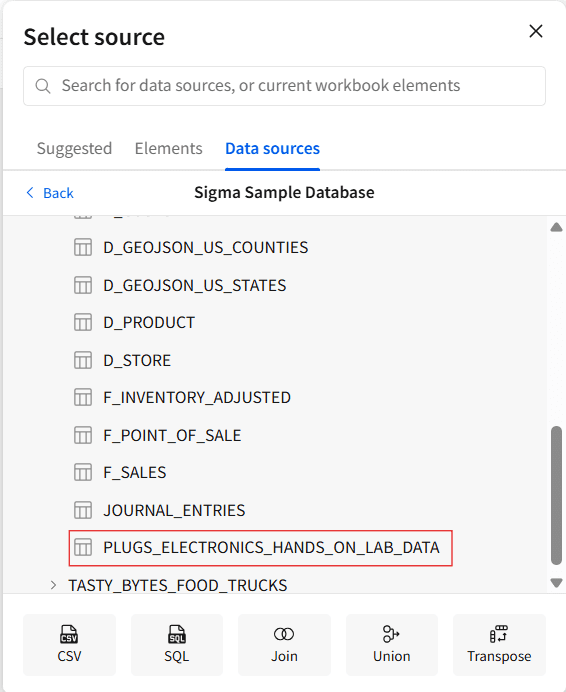
Step 2: Select the data source
From the Data Pane, choose Table. This will open a window where you can browse and select your data source. You can pick from tables in your connected databases (such as Snowflake) or from existing datasets created in Sigma.
In this example, we’ll use Sigma Sample Database > Retail > PLUGS_ELECTRONICS > PLUGS_ELECTRONICS_HANDS_ON_LAB_DATA, then click Open to begin your analysis.

Step 3: Create the chart element
Open the Create Child Element menu (shown below), select Chart under it, and start building a Sankey visualization.

Step 4: Set the chart type
The chart type is set to a bar chart by default; change it to Sankey.

Step 5: Set the first Stage
Set the source columns to specify the stages and categories. In the Stage property, hit + Add column and choose one method from the list below:
For generating stage categories via distinct values present in an existing column, either type in a search or look up the column name in the Select column list and click on it.

- For generating stage categories through a custom formula, choose + Add New column and type the formula in the toolbar.

Step 6: Set the second Stage
In our scenario, we chose the Store Region option from the stage category and followed the same procedure to set up another stage, Store State (at least 2 stages are required to plot a Sankey chart).

Step 7: Add value calculation
In the Value property, click + Add calculation and either select an existing column to aggregate values or choose a new column to create a custom formula in the toolbar. In our case, we created a custom Sales column with the following formula:
Sales = Sum(Quantity * Price)

Step 8: Set the color palette
In the Element properties, click on Color. Here, you can select or create a custom color palette to apply to the category nodes and paths.

The Sankey chart below visualizes sales flow by Store Region and Store State in Sigma Computing.

Here’s the outcome and interpretation:
Left side (Store Region) — Represents the source categories (East, Midwest, South, Southwest, and West).
Right side (Store State) — Represents the destination categories (individual states such as Arizona, California, Florida, North Carolina, Texas, etc.).
Flow bands (links) — Show how sales are distributed from each region to its corresponding states. The thickness of each band indicates the relative sales volume (calculated as
Sum([Quantity] * [Price])).Color intensity — Reflects different magnitudes of sales across connections, helping quickly identify high-performing regions and states.
Example Use Case
One of our retail customers wanted to analyze regional sales by product category. For this, we utilized a Sankey Diagram in Sigma that illustrates sales flow from store locations (East, West, South, Midwest) to product categories (Electronics, Home Goods, Apparel, etc.)
The visualization quickly captured that although the West region had the highest sales, it was the Midwest region that had the most sales for Electronics. This information wasn’t readily accessible in the reports. The client utilized this visualization to redistribute marketing efforts across regions, which improved product availability and sales margins.
Best Practices
Below are the recommended best practices for building meaningful Sankey charts:
- Keep the story simple: Adding more nodes and flows will probably embellish the detail without any better argument for it. 2-3 nodes and 7 primary flows will increase clarity and impact.
- Use interactivity for complex flows: For a more investigative approach, create the Sankey chart interactively when dealing with complex systems and relationships. The chart shouldn’t dictate conclusions; it should provide material for exploration.
Closing
And that’s how to build a Sankey chart in Sigma Computing. Sankey charts are a useful type of data visualization to demonstrate the flow of data between various categories or stages. Not only do they show transitions easily, but they also show patterns, bottlenecks, and the key points of a process or dataset.
Try your hand at this in Sigma, and see how plotting the path of your data will help reveal stories, trends, and smarter decision-making paths.

Ready to take your Sigma dashboards further?
Start incorporating Sankey charts into your key workflows and share them with your team to spark new questions, insights, and decisions.
FAQs
Can I make a multi-step Sankey chart in Sigma?
Yes, we can make a multi-step Sankey chart by adding multiple columns under Stage in chart settings.
How do I reduce clutter in a Sankey chart?
It is recommended to use columns with lower cardinality for each of your stages to reduce clutter.


