

What is a Point-in-Time Metric?
Here are several examples:
- Temperature and weather measurements
- Pending support tickets
- Open claims
- Active devices in IOT data
- Customer accounts in a specific status
- Number of employees assigned to an account
Point-in-time metric values change over time, but you wouldn’t want to sum up those values over time. You would generally aggregate values for these kinds of metrics across most dimensions of the dataset except for date or time.
P.I.T. or P.I.T.A.?
Point-in-time metrics can be more confounding than regular sums and weighted averages when building analytics in Tableau. This is especially true when a point-in-time metric is used as part of another weighted metric, leading to even more complex calculations. I encounter these situations regularly and thought it would be helpful to create a guide and reference for others.
There are a few specific challenges that can arise when working with these metrics which I haven’t seen directly addressed in most other resources.
- What if I need to show weekly or monthly snapshots of the PIT metric, but always show the most recent daily value too?
- What if I need to calculate and display PIT metrics alongside other aggregated metrics with a shared date axis?
- How can I get PIT calculations to play nicely with dynamic date periods and ranges for interactive dashboards?
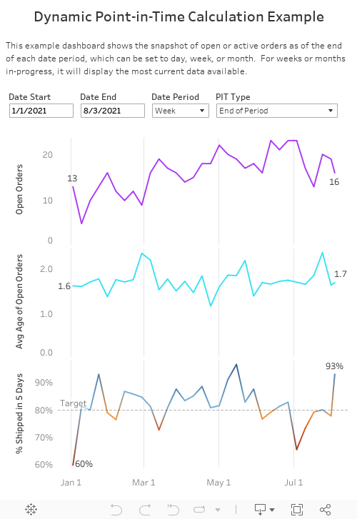
The example I’ll be using here is open or active orders from the example Superstore dataset that comes with Tableau. This could be part of a view for an operations manager who is responsible for ensuring orders are shipped on time and would want visibility into the number of open orders over time, the age of those orders, and service level for shipping times.
Additionally, the structure of the data you are working with may vary considerably, so I’ll be covering two different scenarios, depending on whether your data is pre-aggregated within your source table, or is stored at the record level and needs to be calculated in Tableau.
Here is what I will walk you through:
- Building a point-in-time metric for active order count with a dynamic date axis for either date, week, or month
- Building a weighted point-in-time metric for the average age of active orders corresponding to the first metric.
- Demonstrating four different means of representing PIT metric values grouped across dates (first date of the period, last/recent date of the period, an average of dates within each period, and maximum value within each period)
- How to achieve all of these against either a pre-aggregated data source or a record-level data source with a date scaffold.
Pre-Aggregated Data
First, I’ll cover what you can do when your data already has the point-in-time metric calculated for you. I’ve run the Superstore data through a Tableau Prep flow to get it into this format, which may be typical of how you’d see the data from a data warehouse where the aggregation is defined by upstream integration processes.

Here, open orders over time are already calculated for us, which means less work for Tableau to calculate and a potentially more performant dashboard. However, since we don’t have order-level detail in this table, we can’t immediately build drill-in actions without a second data source. Overall, I try to use the most lightweight data structure I can that meets the report’s requirements.
If you’d like to follow along, feel free to download the example dashboard embedded at the end of this article.
Parameter Setup
Now, let’s set up our parameters. We’re going to create user controls to define the report’s start date, end date, date period (day/week/month), and the method of point-in-time value roll-ups across dates.
Create a regular date parameter called [Date Start] and another called [Date End]. Create a parameter with a string list named [Date Period], with the Date, Week, and Month as the list of values.

Then, create a fourth parameter called [PIT Type] as a string parameter with the following options. Since I want to demonstrate four different ways of rolling up PIT values across a date period, this will let us test all of them with a single set of calculations. Your requirements might differ depending on your own project, so hopefully this will cover most possibilities, or at least get you close to what you really need.

In most cases, you’ll want to represent weekly or monthly rollups for PIT metrics as of the very beginning or the very end of each period. Alternatively, there is also value in using an unweighted average of values across each date in the period, if you want a representation of the overall trend that considers each date equally. Or you may want the maximum value within each period – like if you wanted the monthly high temperature across each date within that month, for example.
Date Calculations
Now that our parameters are set up, let’s build our date dimensions. This data source has a [Report Date] field, against which all other metrics are aligned. This makes things easier for our data design, and I try to get my data prepped this way when possible, and where it makes sense.
Create the following calculated fields, and if you like, put them in a “Dates” folder to keep things organized.
// Report Date Filter

[Report Date] >= [Date Start] AND [Report Date] <= [Date End]
// Date Period Start

DATE(CASE [Parameters].[Date Period]
WHEN 'Date' THEN [Report Date]
WHEN 'Week' THEN DATETRUNC('week',[Report Date])
WHEN 'Month' THEN DATETRUNC('month',[Report Date])
END)
// Date Period End

{FIXED [Date Period Start] : MAX([Report Date])}
This calculation is important and works by referencing the truncated period start date along with the highest individual date within each date period. This lets us reflect on the most recent date of a month or week in progress, which is a common need.
// Date Period (for viz)

CASE [PIT Type]
WHEN 'End of Period' THEN [Date Period End]
ELSE [Date Period Start] END
This is the date dimension we’ll actually use in the viz along the X-axis. Because it looks at the [PIT Type], we can make sure that period end dates are shown in their proper position when the period is incomplete.
Next is the date filter. Create the following calculation, add it to your filter pane, set it to “True” only, and then make that filter a context filter. That step is needed to get the date axis to display the way we want since it filters out irrelevant dates before the LOD calculations are applied.
// Report Date Filter (add to context filters)

[Report Date] >= [Date Start] AND [Report Date] <= [Date End]
PIT Calculations
Now create the following calculations, which will meet the needs of each combination of parameter selections.
// Open Orders PIT

CASE [PIT Type]
WHEN 'Start of Period' THEN
    SUM(IIF([Report Date]=[Date Period Start], [Open Orders],null))
WHEN 'End of Period' THEN
    SUM(IIF([Report Date]=[Date Period End], [Open Orders],null))
WHEN 'Avg of Each Date in Period' THEN
    AVG({INCLUDE [Report Date]: SUM([Open Orders])})
WHEN 'Max of Each Date in Period' THEN
    MAX({INCLUDE [Report Date]: SUM([Open Orders])})
END
Since open orders by date are already provided in the source table, this filters the data to just the appropriate single date within the table for the selected date period and PIT calculation type. For example, if we’re viewing by month and PIT type is set to the end of the period, it will calculate and display the values for just the last date in each month in the date range selected. The last two case options give the average and max value aggregates across the individual dates within each month, or selected date period.
// Average Age of Open Orders PIT

CASE [PIT Type]
WHEN 'Start of Period' THEN
    SUM(IIF([Report Date]=[Date Period Start], [Total Open Order Age],null))
    /SUM(IIF([Report Date]=[Date Period Start], [Open Orders],null))
WHEN 'End of Period' THEN
    SUM(IIF([Report Date]=[Date Period End], [Total Open Order Age],null))
    /SUM(IIF([Report Date]=[Date Period End], [Open Orders],null))
WHEN 'Avg of Each Date in Period' THEN
    AVG({INCLUDE [Report Date]: SUM([Total Open Order Age])/SUM([Open Orders])})
WHEN 'Max of Each Date in Period' THEN
    MAX({INCLUDE [Report Date]: SUM([Total Open Order Age])/SUM([Open Orders])})
END
This is a little more complex and represents a weighted metric that is based on PIT values within the data. What we want to know here is for the Open Orders represented for a given time period, what is the average age in days of those open orders? The field [Total Open Order Age] from the source table gives us the total sum of days that all open orders for the report date have been open since the order was placed, as the numerator of the calculation for the average open order age.
Since it is a PIT metric, however, we use a level of detail (LOD) expression to evaluate the weighted calc for each reporting date, then take either the average or max of those values across each date in the period when rolling those dates up. All other dimensions like region, state, country, etc., are aggregated normally, as expected.
Record-Level Data
Now for the bigger challenge. What if your data is record-level? The example for this scenario is the default dataset for Superstore, which has order and product level records, with the individual order date and ship date in each row. The added challenge here is that the data isn’t just at the grain of order ID in the source table, as each order ID can have multiple products. We’ll be leveraging some LOD expressions to do the heavy lifting here, and I’ll explain how and why each one works.
But first, let’s get the data modeled the way we need it by using a date scaffold. Here, I’m using a CSV file with a big list of dates under a single field named [Report Date]. You might have (or want, if possible) a similar date table in your own database. For the most part, you can make it big enough to cover the possible range of dates into the future for the life of the report. Personally, I try to make everything dynamic when possible to prevent the need for future maintenance and tech debt, and there are some clever ways to create dynamic scaffolds… but that’s a whole other blog post!

Drag the date dimension file table into your data source, and edit the relationship to create a calculation of “1” on both sides of the join. This will create a “cartesian join” where all rows in one table join against all rows in the other table. The reason for this is so we can use regular aggregated metrics alongside our PIT metrics using the same date dimension, as is often needed in operational reporting.
Create the exact same calculated date fields as in the example above, as well as the parameters if you haven’t already. Drag [Report Date Filter] to your filter pane, filter to True only, and make it a context filter, just as before.
Now we have more work to do with the metric calculations than last time since we need to calculate open orders over time ourselves here. The key fields we’ll look at are [Order Date] and [Ship Date]. For our purposes, we won’t count an order as “open” on the same day it shipped, and if it happened to ship on the same day it was ordered, it won’t ever reflect as “open” since it never remained that way overnight.
Create the following calculations:
// Open Orders

IF [Order Date] <= [Report Date] AND (
    [Ship Date] > [Report Date] OR ISNULL([Ship Date])
) THEN [Order ID] ELSE null END
// Open Orders PIT

CASE [PIT Type]
WHEN 'Start of Period' THEN
    COUNTD(IIF([Report Date]=[Date Period Start],[Open Orders],null))
WHEN 'End of Period' THEN
    COUNTD(IIF([Report Date]=[Date Period End],[Open Orders],null))
WHEN 'Avg of Each Date in Period' THEN
    AVG({INCLUDE [Report Date]: COUNTD([Open Orders])})
WHEN 'Max of Each Date in Period' THEN
    MAX({INCLUDE [Report Date]: COUNTD([Open Orders])})
END
First, we’ll define an order as open based on the [Order Date] and [Ship Date] if the [Report Date] falls between under the conditions above, or if the order has no ship date yet at all. If open, then we return the [Order ID] field. Then using our [Open Orders] field, we can use COUNTD() to tally all the unique orders that match our conditions for the PIT roll-up type, just as we did above. Overall it’s very similar to the pre-aggregate approach, with an added step or two.
The next metric gets more complicated, but I will of course walk you through it.
// Average Age of Open Orders PIT

CASE [PIT Type]
WHEN 'Start of Period' THEN
    SUM({FIXED [Report Date], [Order ID] :
        MAX(IF [Report Date]=[Date Period Start]
            AND [Order Date] <= [Report Date]
            AND ([Ship Date] > [Report Date] OR ISNULL([Ship Date]))
        THEN DATEDIFF('day',[Order Date],[Report Date]) ELSE null END)
    })
    /COUNTD(IIF([Report Date]=[Date Period Start], [Open Orders],null))
WHEN 'End of Period' THEN
    SUM({FIXED [Report Date], [Order ID] :
        MAX(IF [Report Date]=[Date Period End]
            AND [Order Date] <= [Report Date]
            AND ([Ship Date] > [Report Date] OR ISNULL([Ship Date]))
        THEN DATEDIFF('day',[Order Date],[Report Date]) ELSE null END)
    })
    /COUNTD(IIF([Report Date]=[Date Period End], [Open Orders],null))
WHEN 'Avg of Each Date in Period' THEN
    AVG({INCLUDE [Report Date]:
        SUM({FIXED [Report Date], [Order ID]:
            MAX(IF [Order Date] <= [Report Date]
                AND ([Ship Date] > [Report Date] OR ISNULL([Ship Date]))
            THEN DATEDIFF('day',[Order Date],[Report Date]) ELSE null END)
        })
        /COUNTD([Open Orders])
    })
WHEN 'Max of Each Date in Period' THEN
    MAX({INCLUDE [Report Date]:
        SUM({FIXED [Report Date], [Order ID]:
            MAX(IF [Order Date] <= [Report Date]
                AND ([Ship Date] > [Report Date] OR ISNULL([Ship Date]))
            THEN DATEDIFF('day',[Order Date],[Report Date]) ELSE null END)
        })
        /COUNTD([Open Orders])
    })
END
This is the tricky one. What we want here is the average age of all open order IDs at the daily level, rolled up according to the [PIT Type] parameter selection. For the first two parameter options, we need to filter for the open order conditions and the PIT type date matching at the same time, as the first inner step within the calculation. Then we grab the max value of the total order aging days by report date and by order ID (since there will be more than one row per order and report date) and sum it all up to get the numerator of our average. The denominator is easy since it’s the same as the open order count from earlier.
For the last two PIT rollup types, we’re taking the same calculation, but removing the condition of matching the first or last report date of the period at the inner level of the calculation. Then we are using a LOD expression to roll up the values for the dates in each period by their average or their max.
Want to pull in other simpler metrics using our [Report Date] field? It’s easy, just make a calculation along these lines:
// Orders Placed

COUNTD(IF [Report Date] = [Order Date] THEN [Order ID] END)
// Orders Placed

COUNTD(IF [Report Date] = [Order Date] THEN [Order ID] END)
// Total Sales

SUM(IF [Report Date] = [Order Date] THEN [Sales] END)
Now you can throw any of these together in a viz using the [Report Date] or [Date Period] field as an axis, and they will all play nicely with each other and even with the other PIT metrics you’ve fastidiously crafted.
Alternatives
“But James,” you ask, “why not use table calculations?” While this is another viable approach for many use cases, there are limitations. Solutions involving table calculations without date scaffolding have the drawback of requiring the use of a date dimension field specific to that metric and its record activation conditions, which may vary from other metrics you need to use in conjunction. It also limits our ability to define specific roll-ups across date periods, which was part of our goal for this exercise. In my view, using a date table with LOD expressions offers more flexibility and fewer headaches. I’m not saying it is impossible without a date table, but for more complex calculations you might just need a vacation to recover by the end of it.
In Conclusion
Now you know how to master point-in-time metrics in your own vizzes, with a little patience! LOD expressions are a powerful tool that allows for robust detail and flexibility in how you create analytics solutions.


