

This blog is a step-by-step guide to help you simulate Tableau’s FIXED, INCLUDE, EXCLUDE LOD (Level of Detail) expression functionality in Sigma, using the Sample Superstore database to investigate period-filtered order sales against unfiltered customer lifetime sales.
Here, we will explore two effective ways to implement LOD functionality:
Approach 1: Without Using Lookup Values
Approach 2: Using Lookup Values
Each approach offers unique advantages depending on your specific use case and the flexibility you need in your analysis pipeline. We will walk through both methods step-by-step, helping you understand when and how to apply them while working with your datasets.
By the end of this post, you will be equipped to confidently choose the right method for your scenario and seamlessly implement LOD calculations to enhance your analytics workflows.
Why Implement LOD Calculations?
Tableau’s FIXED LOD essentially allows one to:
Calculating unfiltered aggregates (e.g., lifetime customer sales).
Compare that with filtered period data (e.g., 2022 orders).
% contribution, segmentation, and deeper customer value analyses.
Sigma does not natively support FIXED LOD, but we can achieve it through:
Filtered base table (Table A) containing period-level data.
Unfiltered aggregated table (Table B) containing lifetime metrics.
Lookup to incorporate lifetime values into the filtered table.
Approach 1: Without Using Lookup Values
Step 1: Connect to the Data
Begin by connecting to the Sample Superstore dataset. We’ll refer to this as our Parent table throughout this blog.
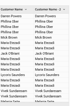
For illustration, you may choose to duplicate the Customer Name column and rename it as Customer Name-2. This step is optional and is only to help visualize column handling during grouping.
Step 2: Create Customer-Level Aggregation
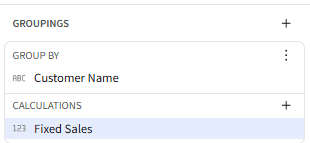
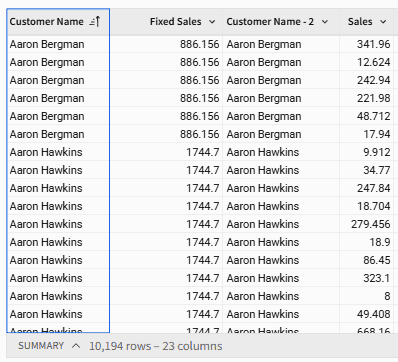
Next, we’ll group the Parent table by Customer Name and calculate the sum of Sales for each customer.
To clearly differentiate, rename this aggregated field as Fixed Sales. This helps you distinguish between your fixed LOD calculation and the original Sales column.
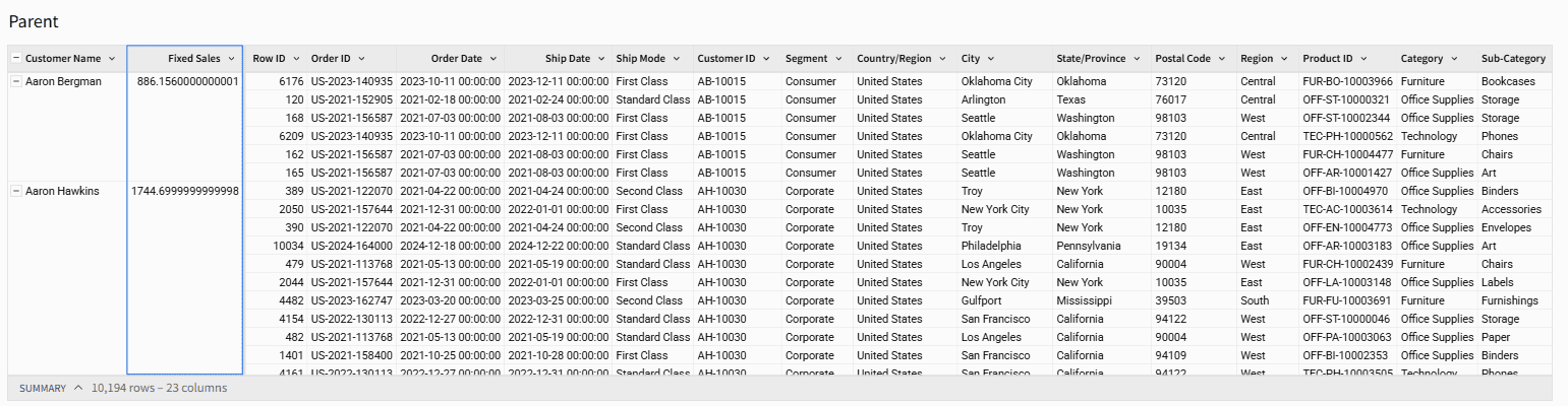
Your resulting table should now display each customer with their corresponding Fixed Sales values.
Step 3: Create the Child Table
Now, create a Child table linked to the Parent table.
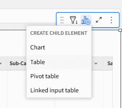
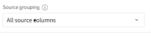
When setting up the child, ensure that All Source Columns are selected in the source grouping options. This ensures you can view and utilize all columns from the Parent table while working in the Child table.
At this stage, you will have a fixed LOD for Sales by Customer Name within your Child table, allowing you to use these values seamlessly in your downstream analyses.
Step 4: Applying Filters
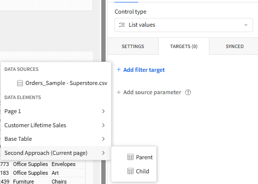
Suppose you want to filter the data by Region. You can add a Region filter and then choose where you want the filter to act:
Context Filter: Target the filter to the Parent table if you want it to act as a context filter, ensuring that your fixed LOD remains consistent within the filtered context.
Dimension Filter: Target the filter to the Child table if you want it to act after your fixed LOD calculation, filtering the results like a standard dimension filter.
Approach 2: Using Lookup Values
Step 1: Create Table A (Base Table)
Source: Sample Superstore dataset.
Columns:
Order Date
Customer Name
Sales
Filters: Add a filter to include only orders from 2022.
Add Sum of Sales aggregation grouped by Order Date and Customer Name.
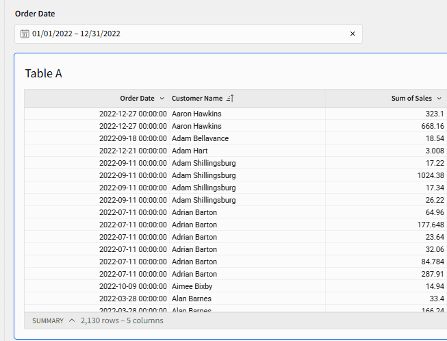
Table A now shows period-level sales at the order level filtered for 2022.
Step 2: Create Table B (Aggregated Table)
Source: Sample Superstore dataset (independent of Table A).
Steps:
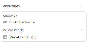
After connecting to the data source, use Groupings:
Add Customer Name in Group By.
Add
SUM(Sales)in Calculations to calculate customer-level lifetime sales.
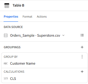
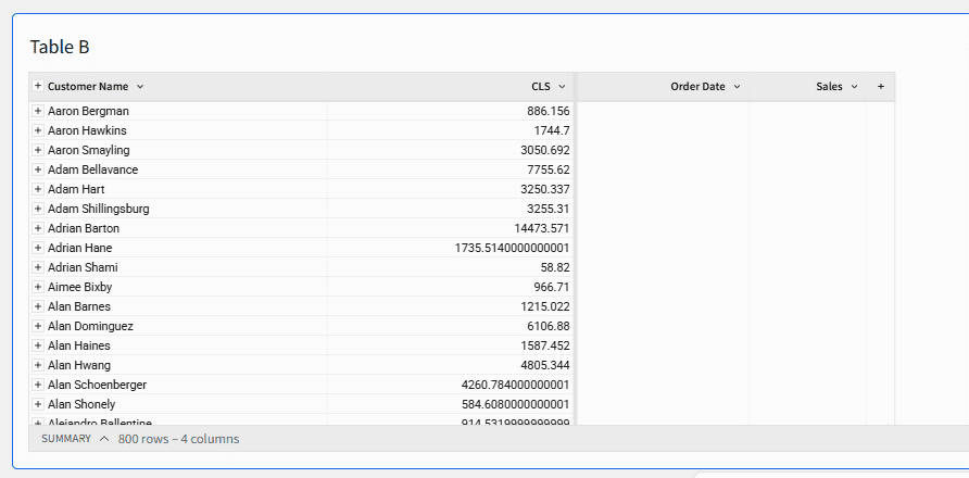
Ensure Table B contains one row per customer (remove Order Date or other row-level fields to avoid duplication).
Columns:
Customer Name
CLS =
SUM(Sales)(Customer Lifetime Sales across all years, unfiltered)
Table B now represents customer-level lifetime sales.
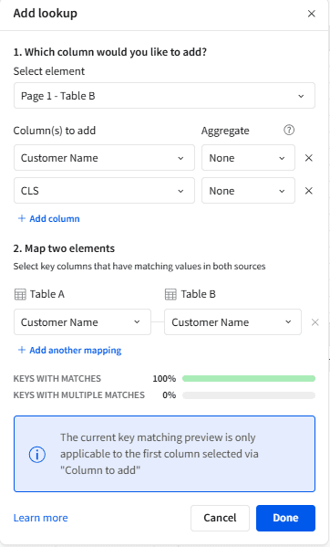
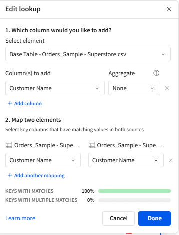
Step 3: Perform a Lookup from Table A to Table B
In Table A, right-click on any column header and choose:
Add Column via > LookupSelect Source: Choose Table B.
Map Key Columns:
Table A: Customer Name
Table B: Customer Name
Column(s) to Add: Select CLS from Table B.
Ensure no aggregation is applied while bringing in the column.
Click Done.
Now, Table A will display Customer Lifetime Sales (CLS) for each order, replicating FIXED LOD behavior.
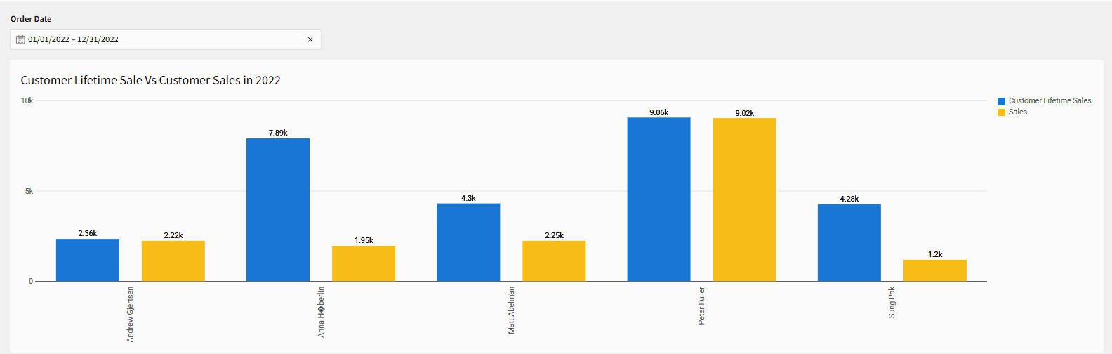
Expected Result:
Table A will have:
Order Date
Customer Name
Sum of Sales (2022)
CLS (Lifetime Sales)
where each order row shows the unfiltered lifetime sales for the customer alongside filtered 2022 sales.
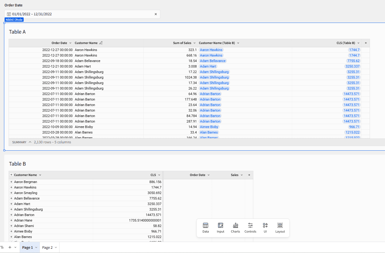
From the table above, we can extract valuable insights, such as comparing customer lifetime sales with their sales in a specific year (2022 in the example below).
Here is another example and some practical use cases for your reference. Using either of the two methods we discussed, you can achieve these results seamlessly in your analysis workflows.
New Customer Acquisition
Steps to Create the Chart:
Start with a base table (Table A) and connect it to the same dataset again as Table B.
Ensure both tables are connected independently (Table B should not be a child of Table A).
In Table B, group by Customer Name and add a calculation for
MIN(Order Date).
Go back to Table A and use a Lookup to add columns from Table B.
Match on Customer Name (ensure no aggregation is selected).
Add
MIN(Order Date)from Table B.
Using Table A, create a bar chart.
X-axis: Weekly
MIN(Order Date).
Y-axis:Count Distinctof Customer ID.Add Region to Color.
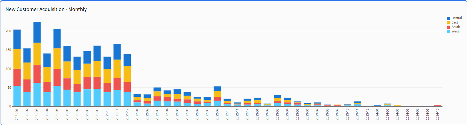
From this chart, you can clearly observe that the rate of new customer acquisition decreases in the later periods.
Since Tableau’s FIXED, INCLUDE, and EXCLUDE LODs can often be used interchangeably depending upon context, the same logic can be employed in Sigma Computing or similar tools to achieve the same LOD behaviors as Tableau.
Conclusion
In this blog, we explored two practical methods to replicate Tableau’s FIXED, INCLUDE, and EXCLUDE LOD functionalities in Sigma using the Sample Superstore dataset:
Approach 1: Using Parent-Child tables with direct groupings and filters.
Approach 2: Using Lookup Values between filtered and unfiltered tables for scalable LOD analysis.
Both approaches help you analyze filtered period-level metrics (e.g., 2022 sales) alongside unfiltered customer lifetime metrics within the same workflow, enabling powerful comparisons and deeper customer analysis without losing granularity.
By mastering these techniques:
You can seamlessly migrate your LOD logic from Tableau to Sigma while maintaining analytical integrity.
You gain the flexibility to handle advanced customer segmentation, contribution analysis, and retention studies within Sigma’s cloud-native, collaborative environment.
You avoid added complexity while building reusable, scalable analytical workflows for your team.
Whether you are transitioning existing Tableau processes or building your Sigma environment from scratch, these methods will ensure your LOD analyses remain strong, consistent, and efficient within your modern BI workflow.

Looking to get even more out of your Sigma experience?
Connect with the experts at phData, we’re here to help you unlock better insights and drive smarter decisions with your data.


