I think it is safe to say that most people are familiar with maps. Today, with a smart phone in nearly everybody’s pocket, the use of GPS tools like Google Maps or Apple Maps is ubiquitous. We use these tools for navigation, finding a new restaurant, searching for a new home, and so much more.
What many may not realize, though, is that maps come in many different types. These types are formally known as map projections, and different map projections are necessary for certain types of presentation or analysis.
The map projection that people are most familiar with is undoubtedly the Mercator Projection, thanks in large part to apps like Google Maps. In recent years, the Mercator Projection has received considerable flak due to its “European bias”—it makes small European countries look much larger than they actually. So, if the Mercator Projection is so awful, why would app designers continue to use it?
The answer is: because the Mercator Projection does what it is intended to do perfectly. The Mercator Projection was originally developed as an aid to maritime navigation. Plotting a bearing due west on the map and following that same bearing in your sailing vessel will take you to precisely where you intended to go. Other map projections fail horribly for the purpose of navigation. The Mercator, as it happens, fails in that it distorts areas increasingly as you move away from the equator.

Because the Earth is a spheroid and maps are flat, there is always some form of distortion in any projection. Some projections, such as Mercator, are known as conformal projections which preserve angles. Other forms of preservation include equal-area projections (e.g., Albers conic) which preserve areas but distort shapes, equidistant projections (e.g., Azimuthal equidistant) which preserve distances between two points, and compromise projections (e.g., Robinson) which attempt to minimize all distortions to make a map that “looks right.”
All of this is preamble to the purpose of this blog post. Much like Google Maps, tools like Alteryx and Tableau utilize the Mercator Projection (more specifically, the Web Mercator, which assumes the Earth is a perfect sphere—this helps to make calculations simpler). But what if your analysis or data visualization requires a projection that conserves area, or shape, or distance?
Thankfully, Alteryx makes updating a spatial file’s projection very easy. Then, with one simple trick (cartographers HATE it!), we can create a map with this new projection in a tool like Tableau.
Updating Projections in Alteryx
First things first: you must have a data set with a spatial object for any of this to work. For this example, I have downloaded a shape file of the countries of the world from GADM.
As I mentioned above, the default map projection that Alteryx and Tableau use is the Web Mercator, which can be seen in the image below.
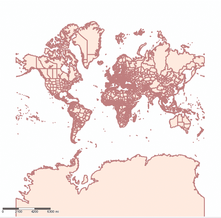
Not only does the Web Mercator distort high latitudes tremendously (note that Russia is actually only half the size of the African continent), but in my opinion it is rather ugly—other map projections simply look better, and this is a benefit that should not be overlooked when building data visualizations.
Once you have completed your workflow, it is time to create a new spatial projection. You do this via the Output Tool. Elect to output your data as an ESRI Shapefile and the configuration menu will look like this:

We are interested in line 4 in the configuration menu: Projection. By default, this option is left blank. We can, however, click on the ellipsis button to the right which pulls up the Edit Projection menu.

Under the Projected Coordinate Systems menu are a lot of map projections. As you will see scrolling through the list, many are built for specific geographic regions, such as Pitcairn Island or Vermont.
Let’s go ahead and pick the Robinson projection—a compromise projection intended to make a visually pleasing world map—under Projected Coordinate Systems→World→Robinson.

At this point we are basically done with the Alteryx portion. Press OK and then run the workflow—that’s it!
The Sneaky Bit
We have now used Alteryx to output a shapefile with the Robinson Projection. However, if you were to open that ESRI Shapefile in Alteryx or in Tableau, the map would look identical to how it was originally (i.e. in the Mercator Projection). What gives?
Tools like Tableau are “smart” enough to re-project the data into Web Mercator. What we must now do it trick Tableau into thinking our data is a Web Mercator without actually changing the projection. So, how do we do that?

We have not mentioned this yet, but when you create a Shapefile you simultaneously generate three other files: DBF (database), PRJ (projection), and SHX (an index file for spatial geometries). What we must do is open the PRJ file and modify its contents.
A PRJ file is a text file that contains information on the manner in which data should be projected. When we told Alteryx to output the data in a Robinson projection, the associated PRJ file (opened with any text editor—I like to use Notepad++) reads this:
					PROJCS["World_Robinson",
GEOGCS["GCS_WGS_1984",
DATUM["D_WGS_1984",
SPHEROID["WGS_1984",6378137,298.257223563]],
PRIMEM["Greenwich",0],
UNIT["Degree",0.017453292519943295]],
PROJECTION["Robinson"],
PARAMETER["False_Easting",0],
PARAMETER["False_Northing",0],
PARAMETER["Central_Meridian",0],
UNIT["Meter",1]]
But, as we mentioned above, Tableau will see this, ignore it, and change the map back into a Web Mercator. So what we must do is change this information so that Tableau thinks it already is in the Web Mercator projection.
To trick Tableau, open the PRJ file in any text editor, delete the contents, and copy the following:
					PROJCS["WGS_1984_Web_Mercator_Auxiliary_Sphere",
GEOGCS["GCS_WGS_1984",
DATUM["D_WGS_1984",
SPHEROID["WGS_1984",6378137.0,298.257223563]],
PRIMEM["Greenwich",0.0],
UNIT["Degree",0.017453292519943295]],
PROJECTION["Mercator_Auxiliary_Sphere"],
PARAMETER["False_Easting",0.0],
PARAMETER["False_Northing",0.0],
PARAMETER["Central_Meridian",0.0],
PARAMETER["Standard_Parallel_1",0.0],
PARAMETER["Auxiliary_Sphere_Type",0.0],
UNIT["Meter",1.0]]
Save the file (do not change the file name), and you’re done! All we have done is replaced the PRJ file with Robinson (or whatever) projection information with projection information from the Web Mercator.
Displaying the Map in Tableau
At this point, all that is left is to build the map in Tableau. Connect to the Shapefile that we created earlier. When you are working with spatial files in Tableau, a new field will appear named Geometry. This is the Tableau equivalent to Alteryx’s SpatialObj field. It is a field that contains the “shapes” of your spatial data.
Double-click on Geometry and add any supplemental fields to the color and detail marks cards to generate a map like the one below.

No matter what new projection you chose, your map in Tableau will look something like this. We have our shapes overlaid on Tableau’s standard Mercator base map. All we need to do from here is navigate to Map → Map Layers and set the washout to 100%.
Keep in mind that Tableau’s built-in map searching functionality will not work with map data in a new projection. Here, for example, if I search for “California” it will zoom into the Pacific Ocean south of where Alaska has been re-projected. But at least the map looks good, and isn’t that all that matters in the end? I encourage you to play around with this technique. Try to find new and interesting map projections that might tell your data story in a new way.

Do you have more questions about Alteryx or Tableau? Talk to our expert consultants today and have all your questions answered!