Evaluating forecast performance is essential in Quick‑Service Restaurants (QSRs), where operational missteps can be costly. Standard accuracy metrics, like Mean Absolute Percentage Error (MAPE) and Mean Absolute Scaled Error (MASE), offer statistical assessments, but often fail to capture the true business cost of errors.
This shortcoming stems from two key problems:
Symmetric error treatment: Many metrics treat over‑ and under‑forecasting equally. But in practice, missing demand during peak hours is far more damaging than slight overproduction during off‑peak periods.
Context‑blind cost structures: Even metrics like quantile loss can’t fully reflect the fluctuating, asymmetric costs tied to time, product margin, or customer impact.
We present a cost‑based framework that integrates contextual cost asymmetry and uncertainty into model evaluation to address these gaps.
Illustrative Scenario: Demand Forecasting at QuickServe Restaurant
Consider QuickServe Restaurant, which is managing demand for its most popular sandwich. Accurate forecasting is essential to balancing inventory costs against potential lost sales.
Forecast Error Type | Example Scenario | Estimated Cost | Interpretation |
|---|---|---|---|
Under‑forecasting | Running out of signature sandwich at lunch | $4–$7 | Lost revenue, goodwill, opportunity |
Over‑forecasting | Unsold sandwich | $2.00 | Marginal cost can be mitigated by using a staff meal |
Suppose QuickServe has two candidate models for forecasting the hourly demand of their sandwich:
Model 1:
MAPE = 15%.Model 2:
MAPE = 18%, anecdotal evidence of fewer peak‑hour stockouts, which could be exceptionally costly.
Standard accuracy metrics favor Model 1. However, management suspects Model 2 might yield better financial outcomes due to its performance profile during high‑cost periods. A method is needed to quantify the cost implications of each model’s error patterns under realistic operating conditions.
Methodology: A Cost‑Based Evaluation Framework
To address this challenge, we decompose the cost of forecast error into distinct components, allowing for nuanced modeling even under uncertainty.
A) Error‑Impact Scaling
g(e): This function defines how the fundamental cost impact scales with the magnitude of the forecast error (e), independent of the specific monetary value or time context. Examples include:
Linear:
g(e) = e. Each unit of error contributes equally to the impact. This is typical of over‑forecasting costs.Quadratic:
g(e) = e². The impact accelerates rapidly with larger errors, which is relevant if large errors cause disproportionate operational disruptions or reputational damage.Dead Zone:
g(e) = max(0, e − D). Errors below a thresholdDhave zero impact, reflecting operational tolerance for minor deviations. Over‑forecasting, which can turn into staff meals, can be considered here.Piecewise: changing slopes after thresholds.
Separate choices may be made for over‑forecasting gₒ and under‑forecasting gᵤ, and should be item and context-specific.
B) Baseline Cost Parameters
Kₒ,Base– baseline $ per unit ofgₒ(eₒ)Kᵤ,Base– baseline $ per unit ofgᵤ(eᵤ)λBase = KᵤBase / KₒBase(relative baseline cost;λBase > 1indicates under‑forecasting is more expensive during “baseline” operating conditions)
C) Dynamic Cost Adjustment κ(conditionₜ)
These multipliers adjust the baseline cost coefficients based on relevant contextual conditions.
κᵤ(conditionₒ,ₜ)– inflates under‑forecast cost when traffic is high, during promos, etc.κₒ(conditionᵤ,ₜ)– inflates over‑forecast cost near closing, limited storage, etc. For the use case of an hourly demand prediction, we set this to be constant at1.
These can be modeled using functions sensitive to the identified conditions, often involving exponential forms such as a log link, for example, log(κ(conditionₜ)) = α + β · conditionₜ, where α and β are parameters reflecting the sensitivity of forecasting errors to certain operating conditions such as traffic. These parameters are also typically uncertain. Setting α to 0 and normalizing the conditions data to be standard normal helps construct distributions for your β parameters.
D) Combined Normalized Loss
Putting it all together, we get a loss function in terms of dollars, but often it is easier to put a distribution on the cost ratio between over‑ and under‑forecasting rather than dollars. In practice, a normalized loss function allows for easier setup while providing the same outcomes; interpretation is in terms of the cost of over‑forecasting during average conditions. The loss for a given forecast at time interval t is given by:
L′(eₒ,ₜ, eᵤ,ₜ, conditionsₒ,ₜ) = κₒ(conditionsₒ,ₜ) · gₒ(eₒ,ₜ) + λBase · κᵤ(conditionsᵤ,ₜ) · gᵤ(eᵤ,ₜ)
We can then sum over the time intervals to get an estimated cost for using a given model.
Addressing Parameter Uncertainty: Monte Carlo Evaluation
Specify distributions for
λBase,α, andβ, for example,λ ∼ Unif(2, 4).Iterate:
Draw one sample of all uncertain parameters.
Compute total cost for each model over a historical back‑test.
Repeat thousands of times to obtain cost distributions.
Compare models on:
Expected cost (mean).
Risk metrics (e.g., 95th‑percentile cost).
Implementing Methodology for QuickServe
We present sample code for implementing this methodology with Python using numpy and pandas (also easily implemented in a PPL like PyMC3).
					import pandas as pd
import numpy as np
import matplotlib.pyplot as plt

df = pd.read_csv("quickserve_history.csv")
# Columns: ['timestamp', 'actual', 'model_1_fcst', 'model_2_fcst',
# 'normalized_traffic']

# Define Error Impact Scaling
def g_over(e_over):

    """Dead zone: first extra unit is free (e.g., staff meal)."""
    return np.maximum(0, e_over - 1)

def g_under(e_under):
    """Linear Cost for Under Forecasting"""
    return e_under

# Dynamic Cost Adjustment - underforecasting is affected by normalized traffic
def kappa_u(traffic, beta_u):
    # k_u(t) = exp(0 + beta * normalized_traffic)
    # At mean traffic this equals 1, so it multiplies the mean cost ratio by 1
    return np.exp(0 + beta_u * traffic)

def kappa_o(): # keep simple: constant =1
    return 1.0

# draw n values from each distribution

# for every std increase in traffic we expect the cost ratio of under to
# overforecasting to increase by a multiple of somewhere between 1 and 2
beta_u_prior = lambda n: np.random.normal(np.log(1.5), np.log(0.5), size=n)

# Baseline cost ratio lambda ~ Uniform(0.5,4) - we think at mean traffic that it
# is between 1/2 and 4 times as costly to underforecast by a unit
lambda_prior = lambda n: np.random.uniform(0.5, 4, size=n)

# Define number of simulations to run and initialize empty cost vectors
N_SIM = 5000
cost_model_1 = np.empty(N_SIM)
cost_model_2 = np.empty(N_SIM)

# Prepopulate errors with vectorized calculations
e_over_1 = np.maximum(0, df['model_1_fcst'] - df['actual'])
e_under_1= np.maximum(0, df['actual'] - df['model_1_fcst'])
e_over_b = np.maximum(0, df['model_2_fcst'] - df['actual'])
e_under_b= np.maximum(0, df['actual'] - df['model_2_fcst'])

for i in range(N_SIM):
    # Draw one value from each distribution and store it
    lam = lambda_prior(1)[0]
    a_u = alpha_u_prior(1)[0]
    b_u = beta_u_prior(1)[0]

    # Calculate cost adjustments for over and underforecasts
    k_u = kappa_u(df['normalized_traffic'], a_u, b_u)
    k_o = kappa_o()

    # Normalised cost per timestamp
    L_model_1 = k_o * g_over(e_over_1) + lam * k_u * g_under(e_under_1)
    L_model_2 = k_o * g_over(e_over_2) + lam * k_u * g_under(e_under_2)

    cost_model_1[i] = L_model_1.sum()
    cost_model_2[i] = L_model_2.sum()

plt.hist(cost_model_1, 40, alpha=0.5, label='Model 1', density=True)
plt.hist(cost_model_2, 40, alpha=0.5, label='Model 2', density=True)
plt.xlabel('Simulated Total Cost (normalized units)')
plt.legend()
plt.show()
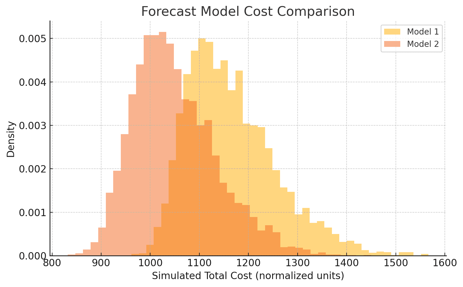
We observe that Model 2—despite having a worse MAPE—shows better financial performance under most simulated cost scenarios. Its distribution has a lower expected value and smaller tails, implying lower average cost and reduced risk.
We can take it one step further and find the expected difference in costs by subtracting the two cost vectors to get the following:
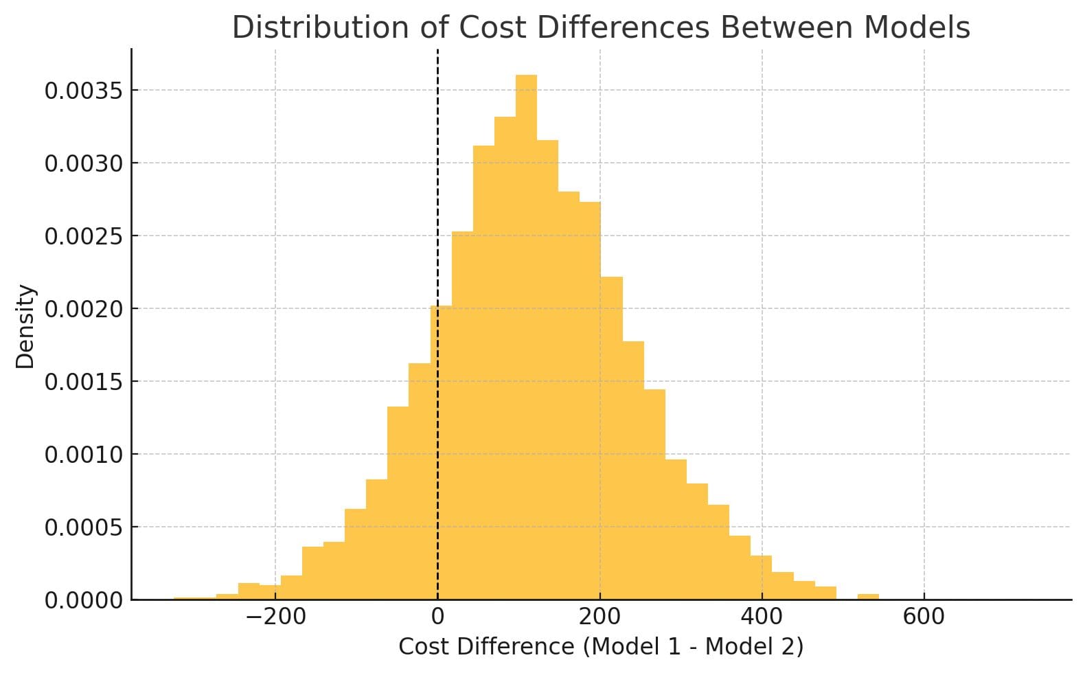
We see that most of the mass is to the right of 0, indicating that for most values of our reasonable cost parameters, Model 2 is better than Model 1. However, we should note that there certainly are values to the left of zero, which would indicate Model 1 being better.
Implication for Stakeholders
Choosing a model with lower statistical error may increase exposure to high‑cost under‑forecasting events. This reinforces the need for domain‑aware model selection, especially in customer‑facing, high‑variance operations like QSRs.
Alternative: Fixed‑Parameter Sensitivity Analysis
Assume:
g(e) = e, κₒ = κᵤ = 1.Evaluate total cost for several fixed
λvalues(1, 2, 3, 5, 10).Inspect which model is cheaper across the plausible
λrange.
Implementation Checklist
- Elicit cost ranges from operational stakeholders. (This is often difficult in practice and is deserving of its own article)
- Select shape functions; start linear.
- Identify key cost‑adjusting conditions (traffic index, minutes‑to‑close).
-
Define priors for
λ,α, andβ. - Run back‑tests & Monte Carlo simulations.
- Compare models via their cost distributions; assess not only expected cost, but also the tails of the distributions (e.g., 95th percentiles).
Conclusion: Shifting the Focus from Accuracy to Impact
This framework moves beyond the narrow lens of accuracy metrics, offering a financially grounded perspective on forecast evaluation. It enables model developers to ask more meaningful questions: What kind of mistakes hurt the business most, and which model minimizes that harm?
By decomposing costs, incorporating uncertainty, and aligning forecasts with real‑world tradeoffs, this approach not only improves model selection but also fosters better cross‑functional communication between data teams and operators.
In short, it’s not just about forecasting better, it’s about forecasting smarter.

Turn Data into Predictive Power
At phData, we help organizations turn complex forecasting challenges into clear, data-driven strategies that drive measurable business impact. Whether you’re looking to refine your model evaluation framework or implement scalable forecasting solutions tailored to your operations, our team of experts can help you forecast smarter. Learn more about how phData can support your data and AI initiatives.